The Upside Potential Ratio 2017 update with this link to:

The Forsey-Sortino Model-1 software 

This dropbox link may ask you to sign in but at the bottom you can skip this step. This zip file contains two files: Forsey-Sortino.exe and a Microsoft VBRuntime.exe.  If you get an error message with F-S Sortino.exe you must install the enclosed VB runtime.exe.

 Frank Sortino and Hal Forsey

The concept developed in this paper was first presented in Pensions and Investments Magazine on 9/26/99, page 22. A paper incorporating this ratio was first published in the Journal of Portfolio Management, Fall 1999 issue. The authors, Frank Sortino, Hal Forsey, Auke Plantinga and Robert van der Meer were all professors from SFSU and Groningen University, who, along with Professor Joseph Messina[1] produced numerous studies over the past 16 years showing superior results of the Upside potential ratio relative to the Sortino ratio, Sharpe ratio and information ratio.  This working paper will update this body of research in preparation for this first release of the Forsey-Sortino Model announced on Linkedin.

Post Modern Portfolio Theory basics

If you want to know how well your manager is doing with respect to accomplishing your goals, then both the return and the risk associated with achieving your goal must be incorporated in the performance statistic. Instead of searching for the manager who had the highest average return over some period of time, those investing for some payout in the future should discount that future payout to present value.  That discount rate separates the good outcomes that achieve the goal from the bad outcomes that identify failure.  In our early work we called this the MAR and later changed it to DTR® for Desired Target Return®. As support for our framework for managing portfolios we initially relied on the emerging field of behavioral finance and the esoteric area of utility theory.

Two of the great pioneers in behavioral finance were the late Amos Tversky, professor of psychology at Stanford University and Nobel Prize Laureate Daniel Kahneman. While Tversky and Kahneman’s work described how investors do behave, Peter Fishburn’s normative utility function [1977] described how investors should behave. Rational investors should be risk averse below the benchmark DTR, and risk neutral above the DTR, i.e., they should have an aversion to returns that fall below the DTR, and the farther they fall below the DTR the more they should dislike them. On the other hand the higher returns are above the DTR the more they should like them. Fishburn showed how this utility function was consistent with expected utility theory.

More recently we found support in an article by Dr. Robert Merton in the July-August, 2014 issue of the Harvard Business Review, who said; “The seeds of an investment crisis have been sown. The only way to avoid a catastrophe is for plan participants, professionals, and regulators to shift the mind-set and metrics from asset value to income. Merton echoes our view that everyone is focusing on the wrong goal and “if the goal is income for life after age 65, the relevant risk is retirement income uncertainty, not portfolio value.”  Merton goes on to make many cogent observations. What we would like to focus on is this quote: “Clearly, the risk and return variables that now drive investment decisions are not being measured in units that correspond to savers’ retirement goals and their likelihood of meeting them. Thus, it cannot be said that savers’ funds are being well managed.” In the spirit of that comment we offer the following:

You can’t manage what you can’t describe so we begin with two different descriptions.

Figure 1

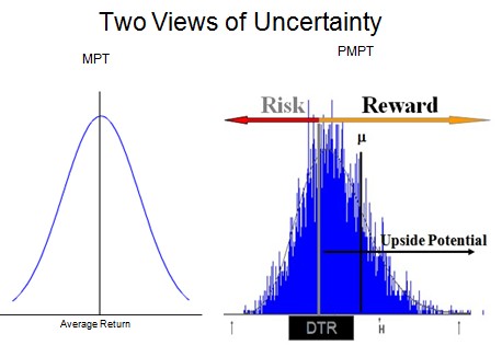
Modern Portfolio Theory (MPT) says that all the statistical characteristics of the portfolio on the left which you are trying to manage can be described by two numbers, the mean (average Return) and the standard deviation of those returns. The framework we developed at The Pension Research Institute, that came to be called Post Modern Portfolio Theory (PMPT), says you need to bring up that asymmetric blue distribution on the right by its bootstraps and then fit to it that black curve you can barely see, called the three parameter lognormal.  Then calculate the mean, standard deviation, upside potential, downside risk and upside potential ratio.

Now let’s examine the three most popular metrics for decision making:

Figure 2

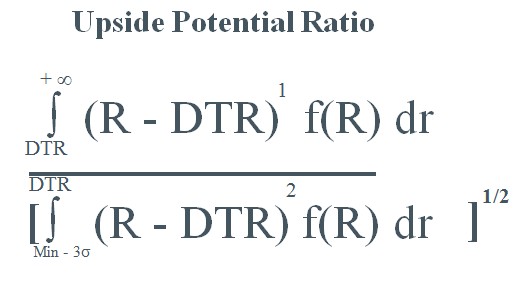
 In Figure 1 all three ratios show the manager’s average return (the mean) in the numerator. The Sharpe ratio compares the mean to a risk-free rate of return.  The information ratio compares the mean to an index return.  The Sharpe and Information ratios do not include a reference to the return (DTR) the investor has to earn in order to accomplish a desired goal.  The Sharpe and Information ratios measure risk in term of standard deviation.  These metrics do not meet the demands of Merton or Fishburn nor the findings of behavioral finance. The Sortino ratio does present a risk-return relationship relative to the DTR.  Now let’s look at the Upside Potential equation:

Figure 3

In Figure 4 we convert the Upside Potential Ratio into a picture that can be more easily understood.

Figure 4

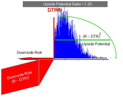
The numerator is more than just the simple differences of two returns as shown in all three of the ratios in Figure 1. Also, It is more than just the probability of exceeding the DTR (shown in blue to the right of the DTR). The upside potential calculation incorporates a magnitude factor that no other ratio has, shown by the green ark that exceeds the upside probability. In the denominator the difference between R and DTR are squared (-4% becomes -16%).  The Upside Potential Ratio presents a very different picture than any of the 3 ratios shown in Figure 1 and it is consistent with the Fishburn utility function.  Unlike any other ratio anywhere, it shows the portfolio has 25% more upside potential than downside risk, which we have shown has more predictive power than the ratios in Figure 1.

An example of the shortcomings of standard deviation and correlations:

Figure 5

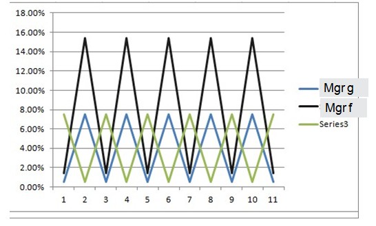
Manager G has much less volatility than manager F and because it has a smaller standard deviation G is less risky than F according to the Sharpe and Information ratios. Also, if we could find a manager with returns portrayed in time series 3 that was perfectly negatively correlated with manager G we could create the MPT version of the Risk-free asset shown in the Sharpe ratio in Figure 2. Many consultants and government agencies might well recommend putting all 401 (k) accounts in the concocted risk-free asset.  But if almost all 401(k) participants need to earn more than 4% to be able to retire with dignity, almost all participants would be guaranteed failure to accomplish their goal.  The Upside potential ratio would not be fooled.

Figure 6 presents a simplified calculation of the upside potential ratio which should never be used in practice. We show this flawed methodology in an attempt to help you understand the concept of upside potential and downside risk and how they differ from the mean and standard deviation.

Figure 6

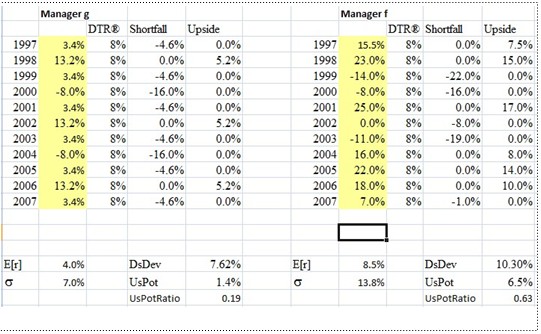
Looking at Figure 6 All MPT believers would say the 4% mean and 7% sigma of G versus the 8.5% and 13.8% numbers of F mean you could only choose between them based on risk-tolerance. Some PMPT believers might say, well, same logic applies using downside risk if you don’t know the upside potential ratio, which is 3 times higher for F. The Sortino ratio gets the sign right but if the DTR was 4% and you earn 4% then the numerator would be zero. But what do you do when both F & G have more downside risk than upside potential as shown in Figure 6?

Let’s say your total portfolio is 75% equity and 25% fixed income and so far this year it is up10%. The market is at an all time high of 2400 on the S&P 500 and the investment committee is considering whether or not to take some profits in equity and increase fixed income.  The DTR given by your actuary is 8% and the expected return is 8% with a standard deviation of 12%.  What does that tell you to aid you in this decision?  Not much.  Suppose you put this information into the Forsey-Sortino Mode as shown in Figure 7.

                                                                 Figure 7

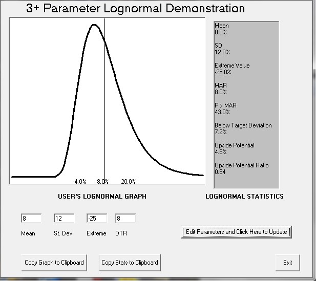
You now see some additional information. The Upside Potential ratio of .64 shows 36% more downside risk than upside potential for the total portfolio.  Might this influence your decision regarding profit taking?  Would you like to be able to change the mean, standard deviation or DTR to see what the impact was? The link at the top will take you to dropbox where you can download it

We will not receive any remuneration. Our only motivation is to provide a tool that might improve the decision making process in portfolio management.

Original References

• De Groot, J. Sebastiaan. “Behavioral Aspects of Decision Models in Asset Management.” Labyrint Publication, The Netherlands, 1998
• Effron, Bradley, and Robert J. Tibshirani, “An Introduction to the Bootstrap.” Chapman and Hall.1993
• Fishburn, Peter C. “Mean-Risk Analysis With Risk Associated With Below Target Returns.” The American Economic Review, March 1977.
• Griffin, M. “The Global Pension Time Bomb and its Capital Market Impact”, Goldman Sachs, Global Research. 1997
• Olsen, Robert A. “Behavioural Finance and its Implications for Stock-Price Volatility.” Financial Analysts Journal, March 1998.
• Sharpe, William F. “Asset allocation: Management style and performance measurement.” Journal of Portfolio Management, Winter 1992.
• Sortino, Frank A. “The Price of Astuteness” Pensions & Investments” May 3, 1999.
• Sortino, F.A., G. Miller and J.Messina “Short Term Risk-adjusted Performance: A Style Based Analysis.” Journal of Investing, Summer 1997.
• Sortino, F. and R.A.H. van der Meer. “Downside Risk.” Journal of Portfolio Management, Summer 1991.
• Statman, Meir. H Shefrin, “Behavioral Portfolio Theory”, Unpublished, Leavey School of Business, Santa Clara University 1998
• Stewart, Scott D. “Is Consistency of Performance a Good Measure of Manager Skill” Journal of Portfolio Management, Spring 1998.
• Tversky, Amos. “The Psychology of Decision Making.” ICFA Continuing Education no 7, 1995

[1] see our first book, “Managing Downside Risk in Financial Markets” p 74, Amazon.com